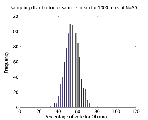
In a previous installment, I showed the results of sampling a population to determine some fact: In that case, it was a hypothetical measurement of the number supporting Obama. By taking 50 "people" at random in the set and tabulating their responses, one gets a rough estimate of the actual proportion of the population who believe something. But how rough? If you run the poll many many times and then tabulate all the results you get, the picture looks something like this:

Sampling distribution polling 50 people, and running 1000 "polls".
The mean of all these poll results was equal to the actual population mean, which is the peak of this chart, at 53.9% in this hypothetical example. So if you were to take a lot of polls and average the result, you'd be damn close to the real value. But if you only take one poll, your result could be as low as 40 and as high as 70. In other words, if you take a poll of only 50 people, and you only do it once, you aren't at all confident of your result.
The chart above shows something which is obtusely called the "sampling distribution of the sample mean". It is a histogram of the results of many samples (polls), which calculate the mean of something (in this case, the mean proportion who want Obama to be president). The sampling distribution of the sample mean itself has a mean! But fortunately that mean is the same as the population distribution, which is what we really care about. However, not all aspects of the sampling distribution are the same as the population distribution.
Characterizing data
If I have a long list of data points, what are the sensible ways to describe this data? The most obvious is the mean. Suppose we poll 10 people on who they want to vote for and get the following results:
| # | Obama | Romney |
| 1 | X | |
| 2 | X | |
| 3 | X | |
| 4 | X | |
| 5 | X | |
| 6 | X | |
| 7 | X | |
| 8 | X | |
| 9 | X | |
| 10 | X |
We could let Obama = 1 and Romney = 0. In that case, we would calculate a mean that would represent the proportion who want Obama to be president. The mean,  , is
, is

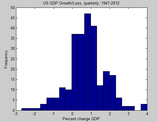
But there are also other times when you also want to know about the spread of the data. For instance, here is the distribution of percent change in US gross domestic product:

Source: St. Louis Fed
The mean looks to be something about +1 (it's actually +0.78), but we might want to also know how often and how much it varies from this. The natural thing would be to add up the differences of each data point from the mean, but if we did that then we'd end up with something close to zero (the mean by definition has roughly as many points above it as below it). Instead, we square the difference from the mean, then take the square root at the end. The standard deviation,  , of
, of  samples is then

where  refers to the set of numbers in your data and
  means "add them all up". For the GDP growth,
  works out to 0.99, meaning that most of the results fall between the mean and 0.99 above and below it, which is clear from the graph itself. Another way of saying it is that the distribution has width that is roughly 2 (plus and minus 1), with just a few points lying outside of this range.
We can calculate the standard deviation for our example poll of 10 people above:

so taking the square root gives  Since the choice between Obama and Romney is just binary, this number has no obvious interpretation as a width of anything, but you can calculate it nonetheless.
Width of the sampling distribution
Let's go back to our original example, a poll of 50 people run 1000 times, which gave us the sampling distribution of the sample mean. The standard deviation for the population is not the same as the width of the sampling distribution!  for the population is about 49.8% (the way of calculating this is simple, but would require a slightly longer discussion to elucidate) but the sampling distribution is much narrower, at just about 7%.
The relationship of the population width and the sampling distribution width is given by the Central Limit Theorem. I'm not going to go into the details of this, but I will state what it says about this case. Suppose our population standard deviation is called  and the standard deviation of our sampling distribution is
  . Then, for sample size
  ,
,

If you want to know the width of the sampling distribution, you take the actual population standard deviation and divide it by the square root of the number of people you sampled. In this case the result is 7 points, so that most of the "polls" show up within 7 points of 53.9% (7 in either direction).
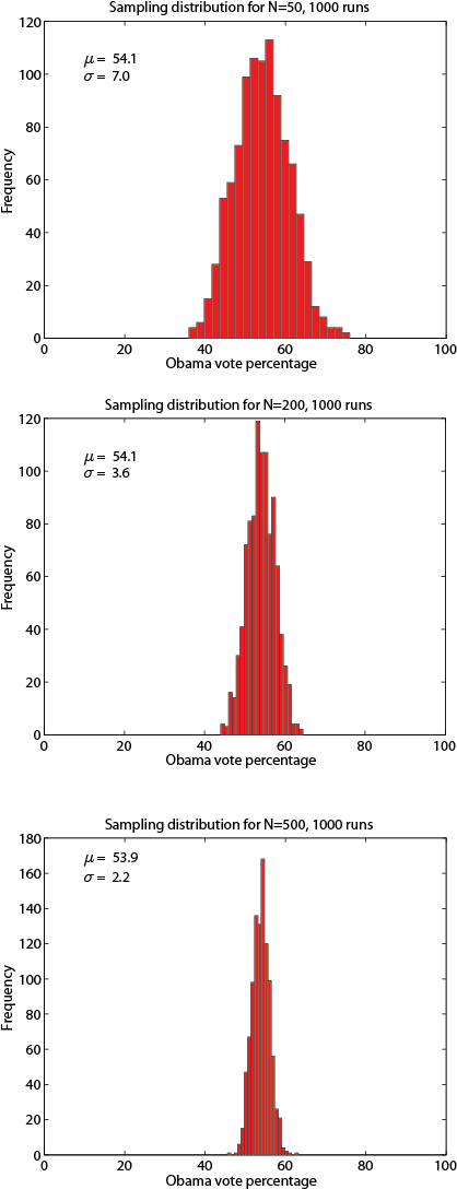
This means that we can be much more confident if we take a larger sample size in our poll. Instead of polling 50 people, suppose we poll 200 people or 500 people, and run the poll 1000 times just like previously. Here are the 3 different distributions, which you can see getting narrower and taller as we increase the sample size:

By  the standard deviation of the sampling distribution is only 2.2. Meanwhile, the Central Limit Theorem predicts

in quite good agreement with the simulation.
What "most" means
What does it mean that if you take a poll of 500 people that the poll result will "usually" be within 2.2 percentage points from the true value? The Central Limit Theorem, in addition to telling us the standard deviation of the sampling distribution, also tells us that the sampling distribution is normal. And for a normal distribution, 63% of all values fall within 1 standard deviation of the mean, 95% within 2 standard deviations, and 99% within 3 standard deviations. If I take a poll of 500 people and get a result that, say, 56% favor Obama, there is only a 1% chance that my result is more than 3 standard deviations from the true value, or within 6.6 of 56. So, we could say "there is a 99% probability that Obama gets between 49.9% and 62.6% of the vote".
A more realistic poll would include something like 2200 people (that's the number Gallup uses in its national tracking poll). Since their  would only be 1 point, they could say, instead, "there is a 99% probability that Obama gets between 53% and 59% of the vote". That's still a 6 point spread, but it's enough to say with confidence that the president will win.
Now, there's a slight issue with this that the reader may have noticed. In order to calculate the probability, one has to already know what the population standard distribution is! Since the only way to do that is to ask every person in the population who they're voting for, this value is always unknown. Instead, statisticians approximate the population standard deviation by the standard deviation that they measure in their poll. If the poll comes up 56 for Obama, the measured standard deviation is 49.6, slightly below the actual population standard deviation of 49.8. Because of the slight error in this, normally we do not say "probability" and switch to saying "confidence". So, we are "99% confident that Obama gets between 53% and 59% of the vote." This range is the confidence interval.
All of this uncertainty in the poll is due to sampling, and it's inherent. The assumption is that you've taken a truly random sample, and in that case you have this much error just from mathematics of randomness. The best designed poll will still have this. However, by averaging a lot of polls together, such as FiveThirtyEight or RealClearPolitics does, you help to reduce this uncertainty even further by increasing  .
.


